What is SWASHES? (Claude)
SWASHES (Shallow Water Analytic Solutions for Hydraulic and Environmental Studies) is a software library and database of analytic (exact) solutions to the shallow water equations (Saint-Venant equations).
It was developed and released by researchers at INRAE (formerly IRSTEA) in France, led primarily by Olivier Delestre and his group.
Official website
https://www.idpoisson.fr/swashes/
(hosted by Institut Denis Poisson, Université d'Orléans)
Background and Purpose
The shallow water equations are the fundamental governing equations used to simulate a wide range of hydraulic and environmental phenomena, including floods, tsunamis, dam-break floods, and river flows. Verification of numerical solvers requires analytic solutions that can be compared against numerical results, but these solutions were previously scattered across the literature. SWASHES was created to consolidate, implement, and distribute them in a single, unified resource.
Main Contents
The analytic solutions included are broadly classified into the following categories:
- Dam-break problems: dry bed, wet bed, 1D and 2D
- Steady-flow problems: hydraulic jumps in channels, flow over bed steps, etc.
- Unsteady problems: Thacker solution (oscillating water surface over a parabolic basin), etc.
- Cases with and without friction: solutions accounting for bed friction such as Manning's law are included
- Rainfall-runoff problems: analytic solutions for surface flow driven by rainfall
Features
- Implemented in C++ and Python and released as open-source software
- Source code: https://sourcesup.renater.fr/projects/swashes/
- Python packages
- PyPI: https://pypi.org/project/swashes/
- conda-forge: https://anaconda.org/conda-forge/swashes
- Python API (pySWASHES) (not recently updated): https://pyswashes.readthedocs.io/en/latest/
- Can be used as a benchmark reference by numerical scheme developers to validate their own codes
- Also published academically as: Delestre et al. (2013), SWASHES: a compilation of shallow water analytic solutions for hydraulic and environmental studies, International Journal for Numerical Methods in Fluids
- Paper (arXiv): https://arxiv.org/abs/1110.0288
- Paper (Wiley / IJNMF): https://onlinelibrary.wiley.com/doi/abs/10.1002/fld.3741
- HAL (preprint): https://hal.inrae.fr/hal-00628246
- INRAE (developer) page: https://www6.val-de-loire.inrae.fr/ur-sols_eng/Productions/Software/SWASHES
※ Some models are not included in the paper above and require consultation of individual publications.
Use Cases
- Accuracy verification of new numerical schemes (finite volume methods, discontinuous Galerkin methods, etc.)
- Validation of well-balanced schemes (testing the balance between bed slope and friction terms)
- Promoting understanding of the shallow water equations for educational and research purposes
SWASHES is widely referenced as a standard benchmark suite in the field of hydraulic numerical computation and plays an important role in assessing the reliability of numerical models.
Setting Up SWASHES
We set up SWASHES using the Python package described above.
The Python environment can be built with Conda using the following command:
conda create -n pyswashes -c conda-forge jupyterlab matplotlib swashesList of Analytic Solutions in SWASHES
We refer to the latest documentation v1.05.00 (2025-04-22).
To download:
- Go to https://sourcesup.renater.fr/projects/swashes/, click the "Docs" tab at the top, then click "doc" in the sidebar and find the latest version.
- Direct link: use the above if this link is broken.
An overview of the analytic solutions included in the latest version is as follows:
- 1D: types 0–9 (inclined plane, bumps, MacDonald, dam break, oscillations, bedload, sluice gates, dam break with step, solute model, mobile rain)
- Pseudo-2D (1.5): MacDonald-type rectangular and trapezoidal channels
- 2D: oscillations, 2D dam, spherical geometry
Details of each analytic solution are shown in the table below.
(Compiled from the manual, though some entries may contain errors.)
| Dim. | Type | Domain | choice | Description |
|---|---|---|---|---|
| DIMENSION = 1 (One-dimensional) | ||||
| 1 | type 0 Inclined plane |
domain 1 L=10 m | 1 | Supercritical flow |
| domain 2 L=20 m | 1 | Transient solution | ||
| 2 | Periodic wave | |||
| 1 | type 1 Bumps |
domain 1 L=25 m | 1 | Subcritical flow |
| 2 | Transcritical flow without shock | |||
| 3 | Transcritical flow with shock | |||
| 4 | Lake at rest, immersed bump | |||
| 5 | Lake at rest, emerged bump | |||
| 1 | type 2 MacDonald |
domain 1 L=1000 m (long channel) |
1 | Subcritical flow — Darcy-Weisbach |
| 2 | Subcritical flow — Manning | |||
| 3 | Supercritical flow — Darcy-Weisbach | |||
| 4 | Supercritical flow — Manning | |||
| 5 | Sub- to supercritical flow — Darcy-Weisbach | |||
| 6 | Sub- to supercritical flow — Manning | |||
| 7 | Super- to subcritical flow — Darcy-Weisbach | |||
| 8 | Super- to subcritical flow — Manning | |||
| domain 2 L=100 m (short channel) |
2 | Smooth transition / shock — Manning | ||
| 4 | Supercritical flow — Manning | |||
| 6 | Sub- to supercritical flow — Manning | |||
| domain 3 L=5000 m (undulating channel) |
2 | Subcritical flow — Manning | ||
| domain 4 L=1000 m (with rainfall) |
1 | Subcritical flow — Darcy-Weisbach | ||
| 2 | Subcritical flow — Manning | |||
| 3 | Supercritical flow — Darcy-Weisbach | |||
| 4 | Supercritical flow — Manning | |||
| 1 | type 2 MacDonald |
domain 5 L=1000 m (with diffusion) |
1 | Subcritical flow |
| 2 | Supercritical flow | |||
| 1 | type 3 Dam breaks |
domain 1 L=10 m | 1 | Wet bed, no friction — Stoker solution |
| 2 | Dry bed, no friction — Ritter solution | |||
| 3 | Dry bed, with friction — Dressler solution | |||
| domain 2 L=20 m | 1 | Self-similar solution, flat bed, laminar friction | ||
| 2 | Self-similar solution, inclined bed, laminar friction | |||
| 1 | type 4 Oscillations |
domain 1 L=4 m | 1 | Planar surface in parabola, no friction — Thacker solution |
| domain 2 L=10000 m | 1 | Planar surface in parabola, linear friction — Sampson solution | ||
| 1 | type 5 Bedload / Exner |
domain 1 L=15 m | 1 | Grass formula |
| 2 | Meyer-Peter & Müller formula | |||
| 1 | type 6 Sluice gates |
domain 1 L=10 m | 1 | Gate opening onto dry bed |
| 2 | Wet bed, free flow, low h_right (= 0.01 × gate size) | |||
| 3 | Wet bed, free flow, h_right = gate size | |||
| 1 | type 7 Dam break with step |
domain 1 L=20 m | 1 | Dam break over discontinuous topography |
| 1 | type 8 Solute model |
domain 1 L=1000 m | 1 | No decay, initial solute concentration |
| 2 | No decay, boundary solute concentration | |||
| 3 | With decay, initial solute concentration | |||
| 4 | With decay, boundary solute concentration | |||
| 1 | type 9 Mobile rain |
domain 1 L=18000 m | 1 | Rain moving at the same speed as the flow |
| 2 | Rain moving slower than the flow | |||
| 3 | Rain moving faster than the flow | |||
| DIMENSION = 1.5 (Pseudo-2D) | ||||
| 1.5 | type 1 MacDonald pseudo-2D |
domain 1 Rectangular short channel B1 L=200 m |
1 | Subcritical flow |
| 2 | Supercritical flow | |||
| 3 | Smooth transition | |||
| 4 | Hydraulic jump | |||
| domain 2 Trapezoidal long channel B2 L=400 m |
1 | Subcritical flow | ||
| 2 | Smooth transition / hydraulic jump | |||
| DIMENSION = 2 (Two-dimensional) | ||||
| 2 | type 1 Oscillations |
domain 1 L=l=4 m | 1 | Rotationally symmetric paraboloid — Thacker solution |
| 2 | Planar surface in paraboloid — Thacker solution | |||
| 2 | type 2 Dam in 2D |
domain 1 L=25 m, l=10 m (≥50 points recommended) |
1 | Parabolic-shaped dam |
| domain 2 L=10 m, l=10 m (≥20 points recommended) |
1 | Cross-shaped dam with central ring | ||
| 2 | type 3 Spherical geometry |
domain 1 α=0 rad | 1 | Global steady nonlinear zonal geostrophic flow |
| domain 2 α=0.406 rad | 1 | Global steady nonlinear zonal geostrophic flow | ||
Running SWASHES
Overview of Arguments
As shown in the table above, most computational conditions for each analytic solution in SWASHES are fixed and cannot be changed. The only parameter the user can modify is the number of spatial divisions (1D: Nx; 2D: Nx, Ny).
At runtime, the conditions from the table above are passed as arguments. Five or six arguments are required:
- arg1: Dimension
- 1: One-dimensional (linear flow)
- 2: Two-dimensional (full planar flow)
- 1.5: Pseudo-2D (MacDonald's method)
- arg2: Type
- arg3: Domain
- arg4: Choice (computational condition)
- arg5, 6: Number of cells
- For 2D cases, also include the number of cells in the y-direction.
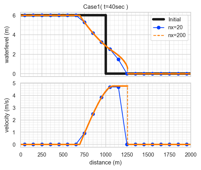
Sample Case 1: "Dressler's dam break with friction"
This is a 1D dam-break problem using the Dressler solution with friction.
The following computational conditions:
- Domain length: L = 2000 m
- Initial water depth: hl = 6 m
- Dam location: x0 = 1000 m
- Chézy coefficient: C = 40 m^(1/2)/s
- Simulation time: T = 40 s
are fixed default values and cannot be changed. Only the number of spatial divisions can be modified.
The model arguments, referring to the table above, are as follows:
- arg1: Dimension = 1
- arg2: Type = 3 (dam break)
- arg3: Domain = 1 (L=2000m) ※ The manual contains an error here.
- arg4: Choice = 3 (Dressler solution)
- arg5: Number of cells = 20 and 200 (two cases)
The execution commands are as follows:
swashes 1 3 1 3 20 > sol11.dat
swashes 1 3 1 3 200 > sol12.dat
The results, when plotted, look like this:
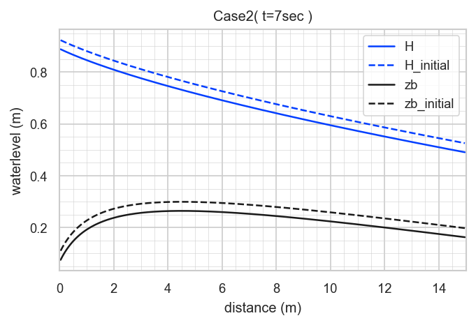
Sample Case 2: "Bedload (Exner) Meyer-Peter & Müller eq."
This case is a bedload transport model accounting for bed variation, using the Meyer-Peter & Müller formula.
The mathematical derivation is highly complex; please refer to:
Berthon et al. (2012), "An analytical solution of the shallow water system coupled to the Exner equation", Comptes Rendus Mathématique, vol. 350, no. 3–4, pp. 183–186.
- DOI: 10.1016/j.crma.2012.01.007
- Preprint: https://arxiv.org/abs/1112.1582
and the SWASHES documentation on bedload solutions: https://sourcesup.renater.fr/docman/view.php/876/21533
The main computational conditions are as follows:
- Domain length: L = 15 m
- Unit discharge: q = 1 m^2/s
- Simulation time: T = 7 s
These are fixed default values and cannot be changed. Many other parameters are also included, and none of them can be modified. Only the number of spatial divisions can be changed.
The model arguments, referring to the table above, are as follows:
- arg1: Dimension = 1
- arg2: Type = 5 (Bedload (Exner))
- arg3: Domain = 1
- arg4: Choice = 2 (Meyer-Peter & Müller eq.)
- arg5: Number of cells = 200
The execution command is as follows:
swashes 1 5 1 2 200 > sol22.datThe results, when plotted, look like this:
Summary
- The library includes some lesser-known analytic solutions, which I personally found very educational.
- The inability to modify detailed computational conditions is a drawback, but the ease with which analytic solutions can be obtained is a significant advantage.
- The computational formulas for each analytic solution are organized in the documentation, making it a useful reference when implementing your own models.
GitHub
https://github.com/computational-sediment-hyd/howtouseSWASHES